RAID Builder *Only RAID Recovery, Network RAID
Overview
RAID Builder makes it possible to assemble complex storages from their constituents in a virtual mode or edit the configurations put together as a result of an automated reconstruction procedure. This mechanism also delivers additional means for the analysis of the array’s raw data, visual representation of its content and layout. Please note that the storages built with its help are just virtual imitations of the real objects. They are processed in a safe-read only mode, without any write operations to the original storage device.
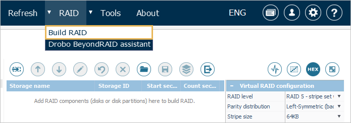
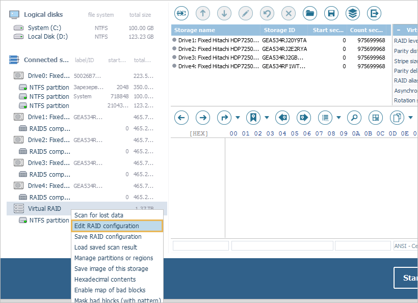
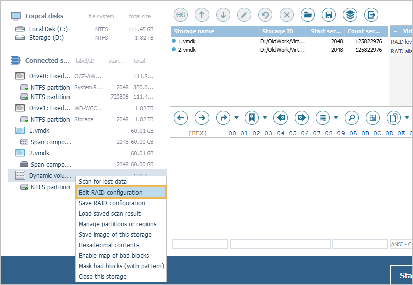
RAID Builder can be launched using the "Build RAID" option of the "RAID" item in the main menu of the program. You can also open it for the already assembled complex storage selected in the storages navigation pane by choosing the "Edit RAID configuration" in its context menu.
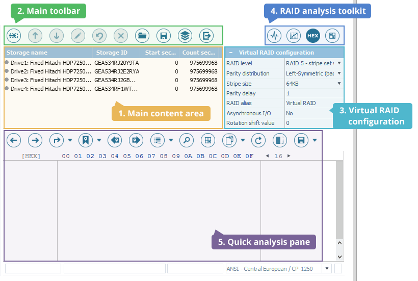
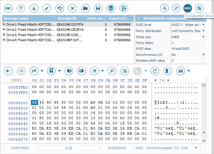
The window itself consists of the main content area (1), the main toolbar of RAID Builder (2) located above it and the "Virtual RAID configuration" section (3) positioned to the right. The toolkit for RAID analysis (4) can be found above the configuration sheet. The bottom of the window contains the "Quick analysis" pane (5) opened by default as context-dependent Hexadecimal Viewer.
-
Main content area
The main content area comprises the list of storages that hold RAID components (physical drives, disk images, other RAID sets, etc.), along with their properties: the name of the source storage and its ID, the starting sector for the component and its overall size in sectors on the given source storage.
-
Main toolbar
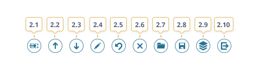
The main toolbar of RAID Builder offers access to the means available for manipulations with the constituents of presented in the main content area. This pane includes the following buttons:
-
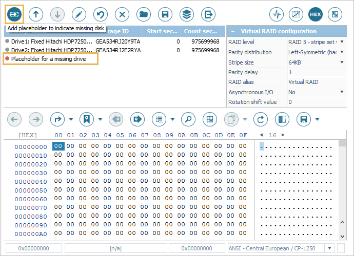
Add placeholder to indicate missing disk
This tool can be used to add a virtual substitute that replaces an absent (failed) component in a degraded RAID set, provided that such an assembly is supported by the employed RAID configuration.
-
Move component up
This tool allows changing the ordinal position for the component selected in the main content area by moving it one step upwards the list.
-
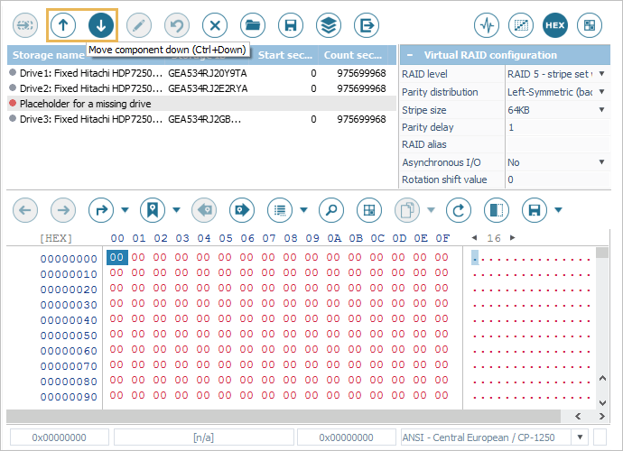
Move component down
Using this tool, you can change the ordinal position for the component selected in the main content area by moving it one step downwards the list.
-
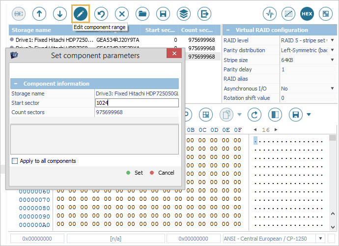
Edit component range
This tool makes it possible to define the range on the storage selected in the main content area (an offset in sectors and the number of sectors following this offset) that will constitute a RAID component. When the "Apply to all components" option is activated, the specified start sector and count sectors values will be used for all storages listed in the main content area.
-
Revert to full size
This option can be used to reset the start sector and count sectors values for the storage selected in the main content area.
-
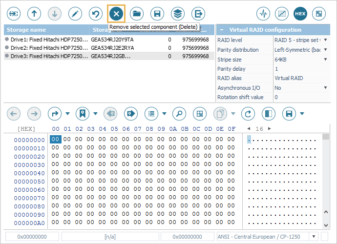
Remove selected component
This tool can be used to delete the selected storage from the list in the main content area.
-
Load configuration from file
This tool allows opening a *.urcf file with the defined RAID configuration that was previously saved in UFS Explorer.
-
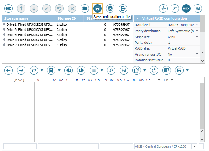
Save configuration to file
This option makes it possible to save the configuration specified in RAID Builder to a *.urcf file for backup purposes.
-
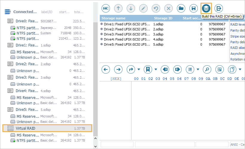
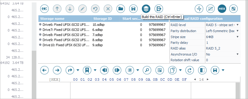
Build this RAID
This tool allows building a virtual complex storage on the basis of the defined configuration. RAID Builder will be closed automatically, and the assembled set will appear in the storages navigation pane. This object can be processed like any stand-alone drive (opened, scanned for lost data, etc.).
-
Close RAID Builder
This option can be used to exit RAID Builder and return to the main screen of the program. Please consider that the currently defined configuration will be lost, unless you save it before leaving.
-
-
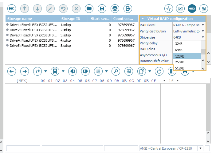
Virtual RAID configuration
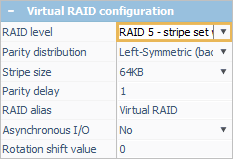
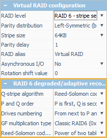
The "Virtual RAID configuration" section is presented as a sheet with a set of RAID properties. Each value can be changed by pressing the "Change value" button next to it and choosing the respective option from the drop-down list, or by selecting the field and entering the value into it manually.
The set of parameters in the sheet differs depending on the selected RAID level, so that only the necessary ones could be specified:
-
RAID level – the type of data distribution scheme used by the complex storage.
-
Parity distribution – the type of algorithm used to allocate the parity information across the components of the array (for RAID 5, RAID 6).
-
Stripe size – the size of a single data block/stripe (for all levels, except RAID 1, JBOD).
-
Parity delay – the number of stripes that fit into a single parity block (for RAID 5 and RAID 6 implemented on certain controllers that employ delayed parity).
-
RAID alias – the name assigned to the assembled complex storage in UFS Explorer (displayed in the storages navigation pane).
-
Asynchronous I/O – the use of parallel data access mode in order to improve performance for large requests on RAID sets with a large stripe size (for all levels, except RAID 1, JBOD).
-
Adaptive reconstruction – the possibility to customize the method of adaptive reconstruction for RAID 1.
-
Data rotation – the type of algorithm used to distribute mirror blocks across the components of RAID 1E (mirror, interleaved).
-
Rotation shift value – the shift of data/parity rotation by the specified value (for RAID 5, RAID 6).
-
Data distribution algorithm – the use of a custom data distribution algorithm specified externally via the RAID Definition Language.
-
LUN – the LUN number on Drobo with multiple LUNs (for Drobo BeyondRAID).
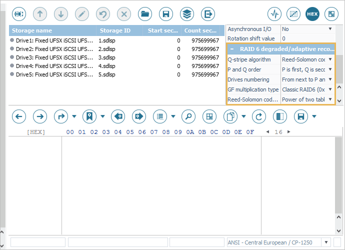
When the RAID level parameter is set as RAID 6, an additional section is presented for configuring the recovery of a degraded/double-degraded array, where and how to obtain parity, etc.:
-
Q-stripe algorithm – the algorithm used to calculate Q-parity blocks in the array.
-
P and Q order – the order in which P- and Q-parity blocks are written.
-
Drives numbering – the order of numeration of the drives for calculation of a Q-stripe (symmetric, asymmetric, including/excluding P and Q).
-
GF multiplication type – the type of multiplication used for calculation of a Q-stripe for a Reed-Solomon code.
-
Reed-Solomon code indexes – the way of calculation of multipliers when computing a Q-stripe by the method of Reed-Solomon.
-
-
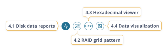
RAID analysis toolkit
This toolkit offers supplementary functionality for easier verification of the consistency of the array being assembled and the correctness of the chosen RAID configuration. It incorporates the following instruments:
-
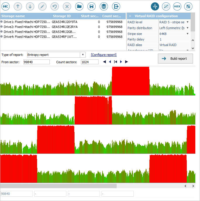
Disk data reports
A dynamic entropy report (histogram) built for each readable component can assist in determining the correct order of drives in RAID. You can change the order of components, so that fragments with high data density should be situated the same way as on the grid pattern of the chosen RAID scheme. It is possible to configure x-scale, y-scale and y-adjustment of the histogram, apply sigma-smoothing to histogram values and pick out custom histogram colors. The report is synchronized with Hexadecimal Viewer to enable immediate navigation to the corresponding hexadecimal position.
-
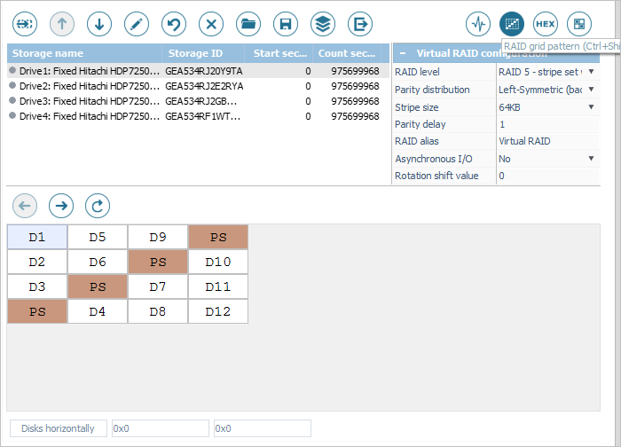
RAID grid pattern
The grid representation of the RAID pattern illustrates the scheme of data/parity distribution among the components of the array (including parity delay, rotation shift, etc.). Using this grid, you can navigate between the stripes or switch to the respective position in Hexadecimal Viewer.
-
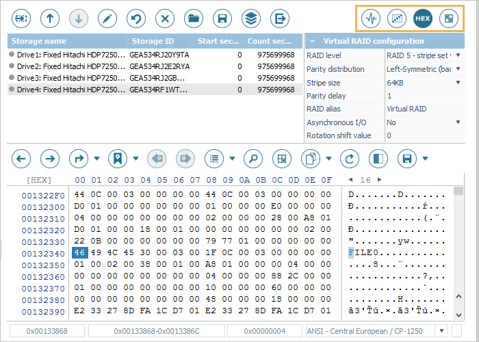
Hexadecimal viewer mode
Hexadecimal Viewer is synchronized automatically with the main content area. When a component is selected, its raw content is displayed in the Hexadecimal Viewer pane. This allows analyzing the on-disk data and visually confirm the order of drives. A switch to another content makes the software show the content of this component at the same position. Hexadecimal Viewer is also configured to allow for "tabulation jumps" of the size of a stripe specified for RAID. More information about the usage of Hexadecimal Viewer can be found in the corresponding section.
-
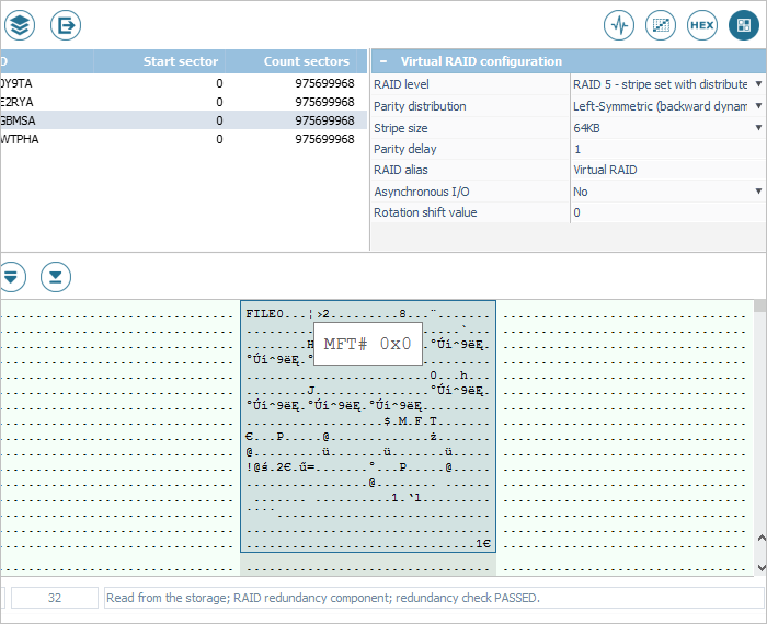
Data visualization
This mode provides visual representation of the RAID data content and enables the indication of various on-disk structures, like MFT or MBR. The mechanism itself is synchronized with Hexadecimal Viewer and can be used to search for the necessary structures by their signatures. The check for parity values and reconstruction of the missing data are performed automatically (when applicable).
-
-
"Quick analysis" pane
The content of this pane is determined by the instrument currently activated in the RAID analysis toolkit. The default tool enabled for analysis is Hexadecimal Viewer.
Automated RAID reconstruction
Certain RAID configurations can be recognized and assembled by UFS Explorer in the automatic mode, provided that enough information is available to determine the correct parameters and the "Detect known RAID" option is enabled in the software settings. The number of drives sufficient to reconstruct the storage depends on the employed RAID layout. Simply use the "Refresh" option from the program’s main menu after connecting the necessary drives.
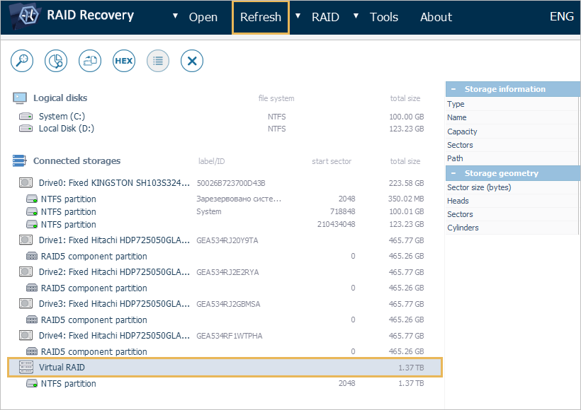
On success, the assembled complex storage is displayed in the storages navigation pane. You can use the "Edit RAID configuration" from the storage context menu to verify the order of components and other properties of the array.
In case of serious RAID configuration damage or other issues, RAID may not be assembled by the program automatically. However, it may be still possible to build RAID in the manual mode by defining the list of its components, their order, level of RAID and other parameters applicable to the given array.
Manual RAID definition
UFS Explorer allows assembling any supported RAID configuration in the virtual mode for subsequent access to its content of or recovery of lost data. The process of manual definition of RAID involves the following steps:
-
Launching RAID Builder;
-
Adding RAID components to the list in the main content area of RAID Builder;
-
Inserting placeholders instead of the unavailable components (if possible for the employed RAID level and supported by the software);
-
Adjusting the accurate order for the given components;
-
Setting up RAID parameters in the "Virtual RAID configuration" section;
-
Putting the parts of the array together in the virtual mode.
Any storage opened in the storages navigaton pane of the program’s main window can be used as a constituent of RAID, including drives, logical volumes, disk images, virtual disks and other complex storages.
Launching RAID Builder changes the default behavior of the items listed in storages navigation pane. You can activate any storage in it, and it will be added as a component of RAID to the main content area of RAID Builder, instead of being opened in Explorer/Partition Manager.
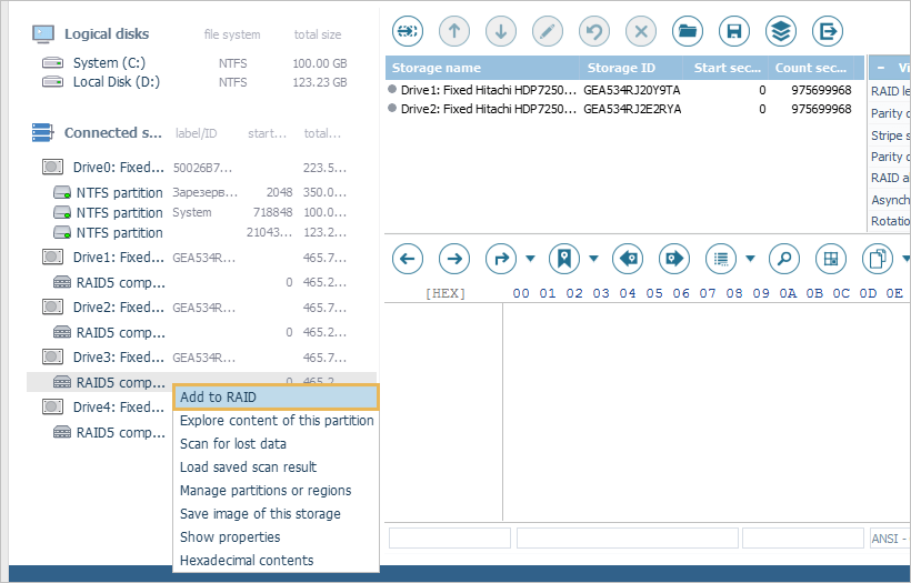
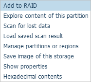
A new option "Add to RAID" also appears in the context menu of each storage.
If a wrong component has been chosen, you can select it in the main content area of RAID Builder and press the "Remove selected component" button in the toolbar or the respective option in the context menu.
For degraded arrays, a virtual disk placeholder has to be added in place of each missing constituent, so that RAID could be built correctly. This can be done using the "Add placeholder to indicate missing disk" button from the RAID Builder toolbar.
To edit the order of storage components, you may select an item in the main content area and use the "Move component up" and "Move component down" buttons to set its correct ordinal position.
If a component of RAID has an incorrect size, or you need to adjust its starting position on the source storage, you can use the "Edit component range" button from the RAID Builder toolbar or the corresponding context menu option. To reset the specified range, use the "Revert to full size" function.
Different RAID layouts use various settings. The "Virtual RAID configuration section" adapts to the selected level of RAID and allows specifying only the required RAID parameters.
For RAID 6 there is an additional parameters sheet related to its parity distribution algorithms. These should be provided only when RAID is reconstructed with missing (failed) drives.
You may use any source materials to find out the correct parameters for your RAID (RAID board BIOS information, configuration files, on-disk structures, device documentation, etc.). Incorrect selection of a RAID type or other settings makes it impossible to recover intact data.
To assemble the array on the basis of the defined configuration, press the "Build this RAID" button from the toolbar of RAID Builder.
In case of successful RAID reconstruction, the array will be added as a new storage to the storages navigation pane. You may apply all the operations available for other storage types (including adding RAID as a component of another RAID) to this RAID. If UFS Explorer detects any valid file systems on it, partition items will appear as its child nodes in the tree of connected storages.
Saving RAID configurations
A RAID configuration can be saved before its assembly using the "Save configuration to file" tool from the main toolbar of RAID Builder.
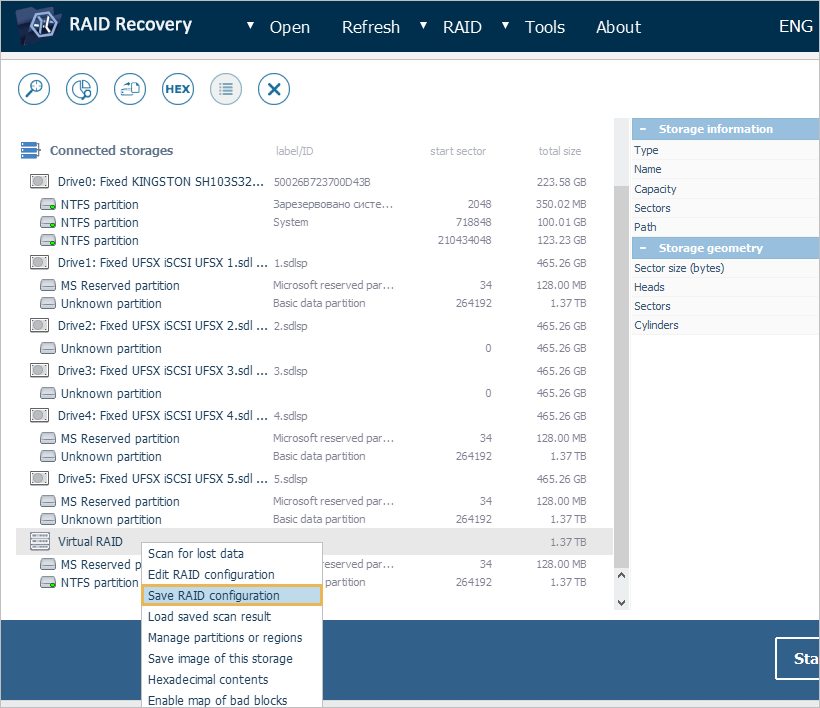
To save the assembled RAID configuration, select the respective complex storage in the storages navigation pane in and use the context menu option "Save RAID configuration".
You may load this configuration in the future from the created *.urcf file using the "Image file or virtual disk" subitem of the "Open" item in the main menu of UFS Explorer.
Correcting RAID configurations
An incorrect RAID configuration assembled in UFS Explorer has no impact on the "real" settings of your device. Still, data recovery from such a RAID set is impossible. For successful accomplishment of the procedure, you have to build RAID with correct parameters. You may perform any number of RAID reconstruction attempts, UFS Explorer does not modify any data on the source disks. Simply choose the "Edit RAID configuration" from the storage context menu, and RAID Builder will be launched again for the given item. Having made the necessary adjustments, use the "Build this RAID" function from the main toolbar of RAID Builder.
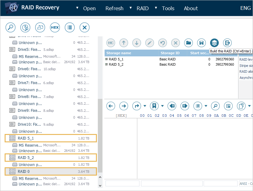
Nested RAID levels
RAID Builder makes it possible to assemble nested (hybrid) RAID sets of different configurations. However, the reconstruction procedure has to be performed separately for each level in the hierarchy.
The assembly is carried out from the bottom to the top: first of all, each RAID unit comprising the lowest level (indicated by the first digit) has to be built as described in the "Manual RAID definition" section.
After the arrays constituting the lowest level are assembled, you will need to launch RAID Builder again and create a new array with the volumes mounted on each of the obtained RAID sets. The type of the final RAID is indicated by the second digit in the employed RAID level.
Composite volumes and non-standard RAID levels
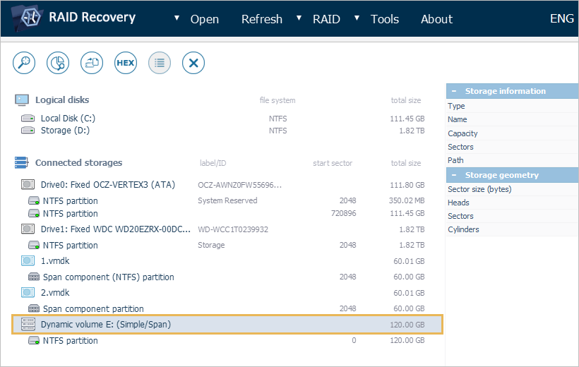
UFS Explorer is capable of working with virtual storages created by various volume managers and other specific solutions. Among the supported ones are Windows Dynamic Disks and Storage Spaces, Apple Software RAID and APFS-based Fusion Drive, Linux mdadm RAID and LVM.
The software can automatically recognize physical components or component disk images as parts of such a composite volume and assemble them accordingly. The result will be displayed as a complex storage in the storages navigation pane with a certain label.
You can use the "Edit RAID configuration" from the storage context menu to check the order of its components or other properties.
In case of metadata damage or other issues, a composite volume may not be assembled by the software automatically. However, it may be still possible to define its parameters manually as described in the "Manual RAID definition" section.
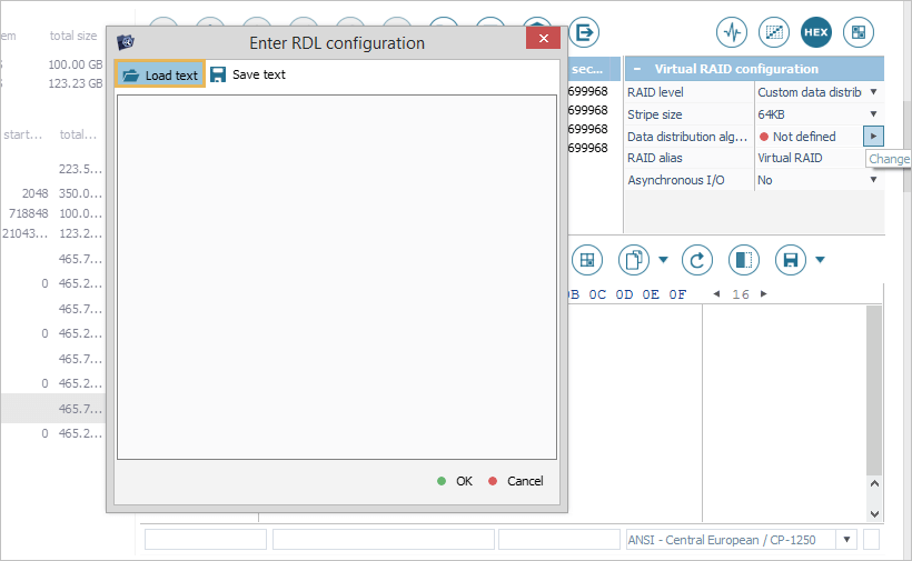
Custom RAID configurations
To apply a custom RAID configuration, you will need to create a text file (ASCII or UTF-8/UTF-16 with a format marker) containing an instruction for the RAID configuration. RAID is configured via the "stripes" command, which uses the "stripe size" and "pattern length" arguments. The command block describes the storage components and their order. The "comma" symbol delimits the components of the same row; the "semicolon" starts the description of the next row. An optional argument for the component defines the row "bias" of the component. The definition is not line sensitive. It's allowed to add block comments /*...*/.
To load the created configuration files, choose the "Custom data distribution algorithm" option from the drop-down list next to the "RAID level" parameter in the "Virtual RAID configuration" section and press the "Change value" button next to the "Data distribution algorithm" property. After successful import of the configuration, the software displays the dialog for its confirmation. If the configuration seems correct, press the "OK" button to accept it. After this, press the "Build this RAID" button in the main toolbar of RAID Builder to accomplish RAID assembly.
Example: RAID 5, Left Symmetric, 64 KB stripe using 4 drives is defined as:
stripes(128,4) {

                            1,2,3;

                            4,1,2;

                            3,4,1;

                            2,3,4;

                            }
Without new lines:
stripes(128,4) {1,2,3;4,1,2;3,4,1;2,3,4;}
Here "stripes(128,4)" defines the configuration with the stripe size of 128 sectors and the pattern size of 4 stripes. Enumeration in {...}-block defines the ordinal number of components. A semicolon defines a new pattern row.
Using the bias argument, you can write the same as:
stripes(128,4) {1,2,3,4(1),1(1),2(1),3(2),4(2),1(3),2(4),3(4),4(4)}
Instead of a component, you may also specify a functional expression. The supported expressions include "reconstruction by parity", "reconstruction by Reed-Solomon code" or "combined by parity and Reed-Solomon".
The formats of functional expressions:
Parity: P{1,2,3}. Here: P – parity function, enumeration – components used to calculate parity.
Reed-Solomon: Q(5,g,4){1,2,3;1,2;3}. Here: Q – Reed-Solomon code, 5 – disk ordinal number, location of Q-stripe, g – index type, 4 – missing drive index; enumeration – disk numbers followed by disk indices (separated with semicolon) to calculate Reed-Solomon code.
Parity and Reed-Solomon: PQ(6,7,i,4,5) {1,2,3;1,2,3}. Here: PQ – combined calculation, 6 – P-stripe drive ordinal number, 7 – Q-stripe drive ordinal number, i – index type, 4 - disk index to reconstruct, 5 – disk index of the second missing drive; enumeration – disk numbers followed by disk indexes (separated with semicolon) to calculate Reed-Solomon code. Index type g – two power of index in Galois field, i – just a simple index.
Samples of RAID configurations with reconstruction:
a) 4 x RAID 5, Left Symmetric, 64 KB stripe, without drive 3:
                            stripes(128,4) {

                            1,2,P{1,2,3};

                            3,1,2;

                            P{1,2,3},3,1;

                            2,P{1,2,3},3;

                            }
b) 5 x RAID 6, Left Symmetric, 64 KB stripe, without drive 3, redundancy order is P, then Q:
                            stripes(128,5) {

                            1,2,P{1,2,3,4};

                            4,1,2;

                            3,4,1;

                            P{1,3,4},3,4;

                            2,P{2,3,4},3;

                            }
c) 5 x RAID 6, Left Symmetric, 64 KB stripe, without drives 3 and 5, redundancy is P, then Q:
                            stripes(128,5) {

                            1,2,P{1,2,3,4};

                            Q(3,g,1){1,2;2,3},1,2;

                            3,P{1,2,3},1;

                            PQ{1,2,g,1,3}{3;2},3,PQ{1,2,g,3,1}{3;2};

                            2,Q(1,g,2){2,3;1,3},3;

                            }
If RAID has a "parity delay", you may specify a "loop" to the entire column, including functional expressions, using the "repeat" function.
For example, 4 x RAID 5 Left Asymmetric, 16 KB stripe size and parity delay of 16 stripes:
                            stripes(32,64) {

                            repeat(16){1,2,3};

                            repeat(16){1,2,4};

                            repeat(16){1,3,4};

                            repeat(16){2,3,4};

                            }
Specifying disks
An optional "drives" section. If the section is not specified, RAID Builder will use the already defined components. If specified, the list of components from RDL will replace the list in the main content area of RAID Builder. The supported types of components are: "disk" – a physical drive, "image" – a disk image file, "span" – a pre-defined span of components. A component is defined as a type (identification information, start offset, use size). The "start offset" and "use size" parameters are optional.
Example:
                            disk (1,2048,233432);

                            image(C:/image1.img,0,4096);

                            image(C:/image2.img);

                            span(myspan01,0,40960);
Physical drive identification information under Windows is the ordinal number of the drive; under macOS, Linux, etc. – the full path of the block device, for a disk image – the full path of this disk image, for a spanned volume – its identification name.
Here is an example of a full configuration for HP RAID with 4 x RAID 5 Left Asymmetric, 16 KB stripe size and parity delay of 16 stripes:
                            drives {

                            disk(1,1088);

                            disk(2,1088);

                            disk(3,1088);


                            disk(4,1088);

                            }

                            stripes(32,64) {

                            repeat(16){1,2,3};

                            repeat(16){1,2,4};


                            repeat(16){1,3,4};

                            repeat(16){2,3,4};

                            }
If a configuration contains only the "drives" section, it simply loads the components into RAID Builder, without defining any RAID configuration.
Defining SPAN
A span can be defined with the help of the "defspan" section. It must be defined before being used as a component. The syntax of the span definition is: defspan(name){enumeration}. Enumeration may include the same components as for the "drives" section (including spans).
Example:
                            defspan("myspan01") {

                            disk(1,2048,233432);

                            image("C:/image1.img",0,4096);


                            image("C:/image2.img");

                            span("myspan00",0,40960);

                            }
A simple span can be loaded via RDL using the following code:
                            defspan("images") {

                            image("C:/image1.img");

                            image("C:/image2.img");

                            image("C:/image3.img");

                            }

                            drives {

                            span("images");

                            }

                            stripes(1,1) {1}